OVERVIEW

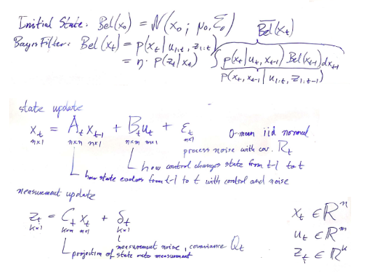
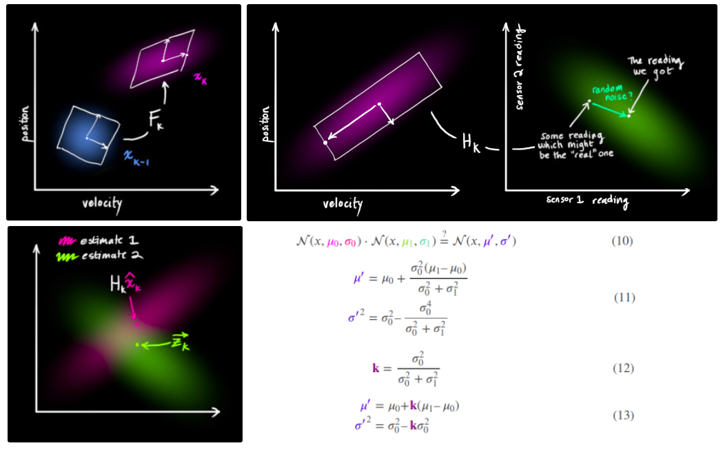
Kalman filter is a Bayesian filter with Markov assumption, which is decompose into two parts: prediction and measurement. The prediction part can be initialze by GPS with some initial uncertainty. This uncertainty is subject to external motion noise, which is assumped to be a zero-mean guassian that’s mutually independent with the process noise itsel, and therefore it does not coupled with state vector x in the expected variance. Furthermore, we use our prediction to describe the distribution that our sensor is reading from, which itself is also subject to the sensory noise. Note that our prediction could be off i.e. the actual distribution of state is NOT a guassian, but it’s modeled this way for the consistnecy of our model. Sometimes, the measurement process is also referred as correction process.

Now, to reconcile our belief, the two gaussian distribution were multiplied together to form a new gaussian distribution. The detailed derivation of muiltiplication of two gaussian function is described here. Looking at the formula, one should realize that Kalman update would always reduce the variance of the estimated state variables, in the best case scenario where sensory variance R = motion variance Q, the variance could be reduce by 50% (30% in standard deviation). Variance of Q, R determines which guassian distribution to trust more, which in practice are often guesstimated. A really great, illustrative explanation of Kalman filter is available at this blog.

Application in Human Position Tracking

Kalman filter can be used to devlope a human-following robot by constantly mapping the human position (x,y) from sensory laser frame back to the global origin. The Kalman filter provides robustness in temporal occulsion by omitting sensor input and thus the variance in prediction grows larger and larger. The nearest human position within standard deviation of prediction center is assigned to be the target. The challenge arise from modeling the motion model, since the linear model would quickly fail when the target human make a turn. To address this issue, a quadratic at^2+bt+c function was fitted to the past N observed positions, with a reprents acceleration and b represents velocity in the linearized matrix. The same function is used to predict the human position in case of occulsion, and the linearized transition matrix F is used to propagate the covariance matrix. Note that the matrices where time dependent in this approach. In a nut shell, this approach is doing linearization at every timestamp, with the assumption that the linear approximation would hold up for the non-linear states, which depends on the sampling rate, relative velocity and the nature of the motion. Specifically, a quadratic function assumes constant acceleration and smooth velocity transition profile, which could be break when a sudden back-and-forth motion is presented i.e. big jerk and change in acceleration. Note that both R and Q are determined arbitrarily in this application. The motion variance Q could be estimated by first fitting a guassian to the past N positions, then derived its covariance matrix.

Sensor Fusion

Depending on the physical metric of sensory inputs, different ways can be adopted to fuse the inputs

1. Different metric: e.g. acceleromter and gyroscope, the acceleromter can be directly plugged into the transition matrix F making it time dependent; the variance term need to be updated w.r.t physical model i.e. V += t^2 * R_{acc} The the gyroscope is used for correction as usual.
2. Same metric: e.g. position measure by lidar, radar and GPS, chain the update steps, use the updated result of last step as new prediction and reduce the variance sequentially.
   Some reference post

EKF

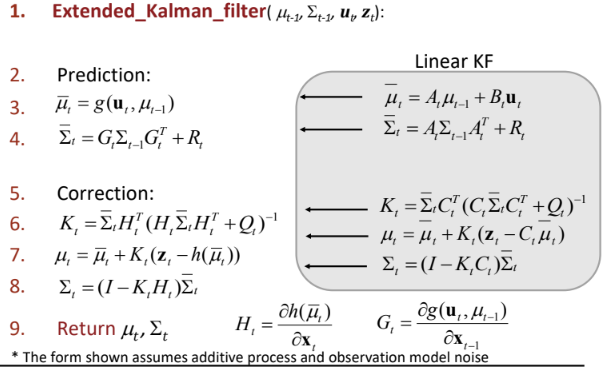
Extended Kalman Filter is an approximation for the non-linear system, where the transformation function f and observation matrix h are non-linear. The solution is to linearize f (hereby denoted as g) and h w.r.t mean, so as to propogate uncertainty i.e. covariance matrix. Note that, in the below equation (3) and (7), non-linear functions are still applied for better mean estimation, only the covariance update make use of the linearize matrices. Such linearization is most appropriate when the uncertainty is small, otherwise the transformed distribution would be significantly different from the true one.

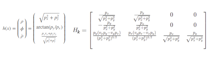
Here’s an radar example of the linearize observation matrix H, note that observation matrix is the mapping from motion prediction to sensor reading, so the matrix is linearized w.r.t state vector x instead of reading y.

UKF

Instead of linearizing then transform, UKF fist transform the sample points then reconstruct the gaussian distribution.

Remarks

1. Kalman filter is proved to be the optimal solution for linear systems.
2. Depending on the state that the Kalman filter is tracking, the variance of the target state may or may not be reduced e.g. convergance on velocity will still lead to unbounded uncertainty of position
3. A quick way to examine whether Kalman filter is working or not is by examing whether the variance has decreased after an update or not
4. Compared to particle filter, Kalman filter could be more robust to high temporal sensory noise, since it still has the motion part to anchor the estimation, while high senosry nosie could throw off all the good candidates for PF and lead to bad convergance.
5. For applications with multiple possible initialization e.g. indoor localization, particle filter is better